Disclaimer: This blog is my attempt to primarily document and organize concepts that I teach to myself, and in no way is it guaranteed that the reasoning developed in my posts is error-free. Through my blog I aspire to let all these ideas mature while receiving constructive feedback, eventually developing intuition. I warmly welcome constructive insights, and discussions so let’s keep this a friendly, respectful space for learning and knowledge sharing. Your contribution highly matters to me and is appreciated!
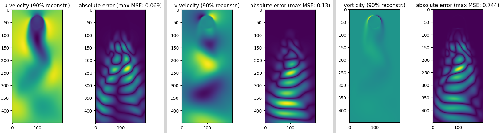
Fluid flow past a cylinder – 90% of energy reconstructed.
Data source: cwrowley/ibpm – IBPM code
K. Taira and T. Colonius. The immersed boundary method: A projection approach. J. Comput. Phys., 225(2):2118-2137, August 2007.
Today I would like to share with you an easy and straightforward application of the SVD on time series for 2D fluid flow past a cylinder.
First, we obtain the dataset using the IBPM code. The data consists of $151$ time samples of $449\times199$ images for the horizontal velocity $u$, vertical velocity $v$ and vorticity.
For each of the features $u$, $v$, and vorticity, the time series is shaped into a $89351\times151$ matrix; that is, the rows of the 2D images are flattened into one dimension. We shall construct our data matrix $A$ by “stacking” the flattened features into a $268053\times151$ matrix.
Original data movie (reshaped into $449\times199$ matrices).
We can apply SVD on the flattened data $A$:
$A = U\cdot\Sigma\cdot V^*$
As we explained in our previous blog post, as matrix $A$ is not square, for the structure of $\Sigma$ we have:
$\Sigma = \begin{bmatrix}\text{diag}(\sigma_1,\dots,\sigma_r) & \mathbf{0} \\ \mathbf{0} & \mathbf{0} \end{bmatrix}$, where $r$ is the rank of matrix $A$.
To this end, let us plot the singular values of $A$, from the diagonal elements of $\Sigma$:
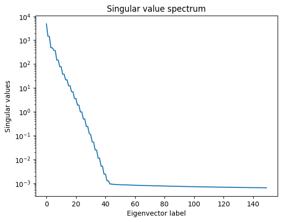
Singular values of matrix A in semilog(y) plot.
The singular values act as a measure of “strength” (or importance) of a combination of a specific pattern across features (indicated by $u_i$) and a specific pattern of measurements across time (indicated by $v_i^*$).
In this case, it can be observed that there appears to be a sheer drop in importance between feature and time patterns after the 42nd singular value. We also notice a large discrepancy of time-feature pattern combination importances even among these first 42 singular values! This leads us to anticipate an even fewer number of singular values to cumulatively capture a large portion of the total energy of the data matrix.Let us plot the most dominant 42 feature patterns for the velocity across the vertical direction $u$:
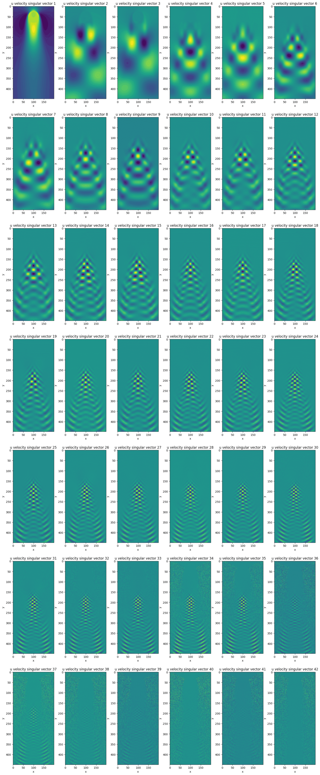
As we can see in the above picture, the first 42 rows of $U$, corresponding to the most dominant 42 feature patterns, can accurately capture the patterns in vertical velocity, although it also appears to have captured unrelated patterns which may be attributed to noise in the measurements. In other words, the presence of noise in the data measurements can lead to data patterns unrelated to the physical process to be additionally captured. It is important to be able to recognise such erroneous patterns when analysing tendencies in the process under consideration.
In our case, we can observe that from the 32nd most dominant feature pattern onwards, noisy patterns also begin to be captured. As the above picture by itself does not give us any information on the “strength” or importance of each feature pattern, we shall introduce an important measure of relative importance, which is even more convenient than merely observing the singular values as we previously did.
To this end, we introduce the relative energy contributed by the singular values up to the most dominant $i$ values, based on the Frobenius norm:
$ E_i = \frac{\sum_{k=1}^i \sigma_{k,k}^2}{\sum_{l=1}^r \sigma_{l,l}^2} $
This metric of energy contribution can help us analyse which tendencies truly matter even more easily, as it is a normalized (meaning that the contributed energies are always compared to the maximum attainable value of 1), and also a cumulative measure (meaning that we get total contribution in energy up to $i$ dominant values).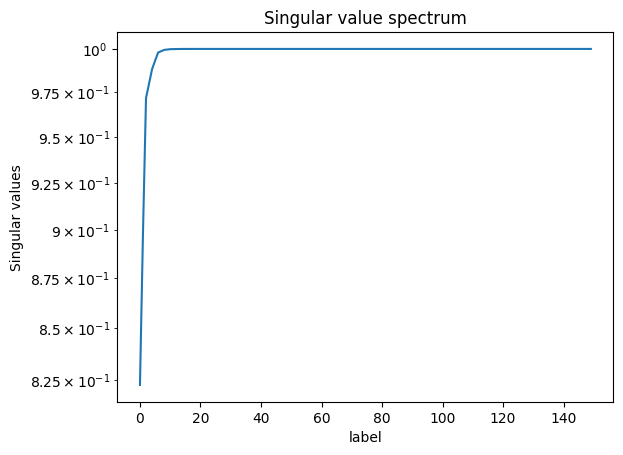
Spectogram of the data’s singular values.
We notice that $\approx99.9%$% of the movie’s energy is recovered using the most prevalent 10 singular values, while $\approx90.0%$% of the movie is recovered using the most prevalent 6 values.
As can be noticed, the reconstruction of the original movie up to $\approx99.9%$%of the original data energy leads to a much smaller mean squared error compared to reconstructing the movie up to $\approx90.0%$% of the original energy.